Overview

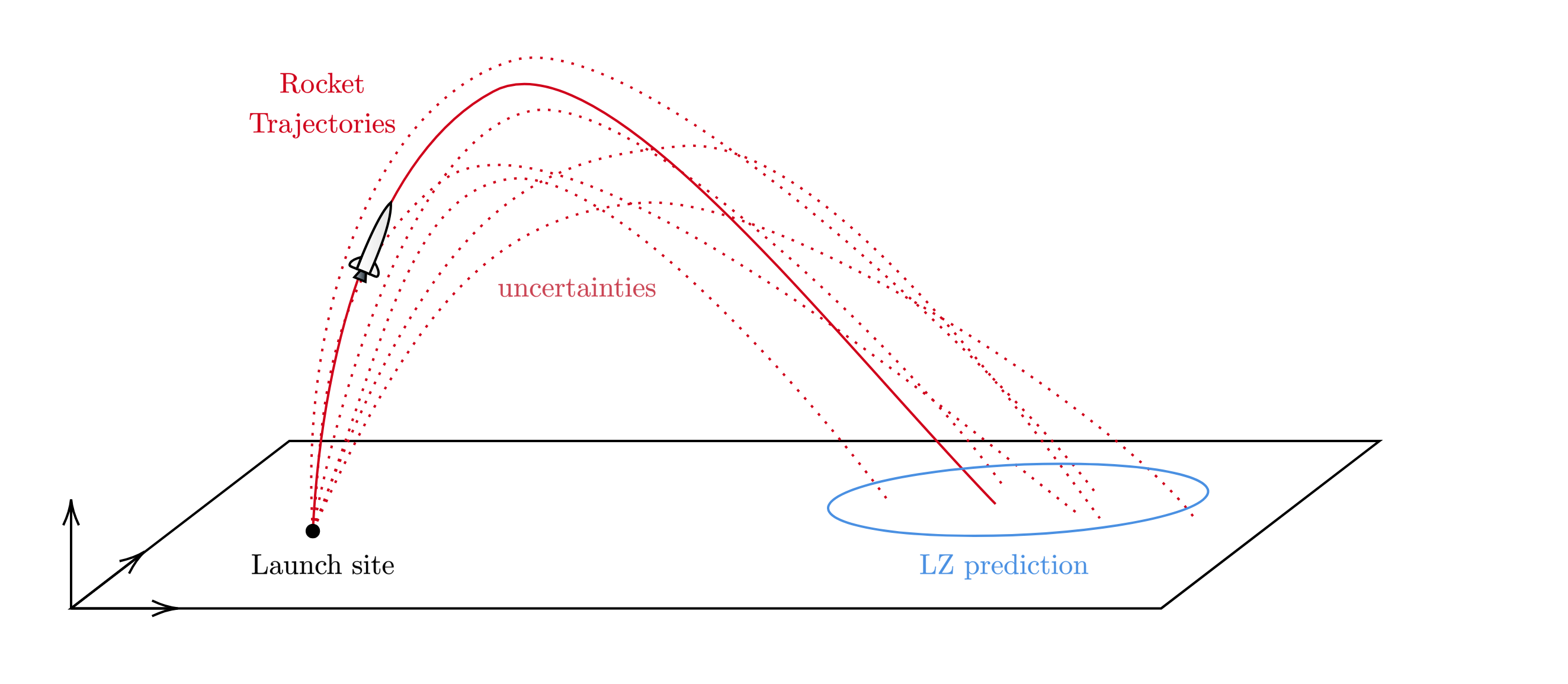
The goal of this project was to learn more about the applications of statistical mechanics and numerical schemes for partial differential equations. The idea started as a personal side-project when working on the DARE rocket simulation software for the Stratos V rocket. The main idea is that instead of running millions of simulations of the dynamics of a rocket, each with varying initial conditions and noise, we run a single simulation of the probability distribution of states over time. This could be used for apogee or landing zone prediction of a rocket under different conditions.

Technical Details

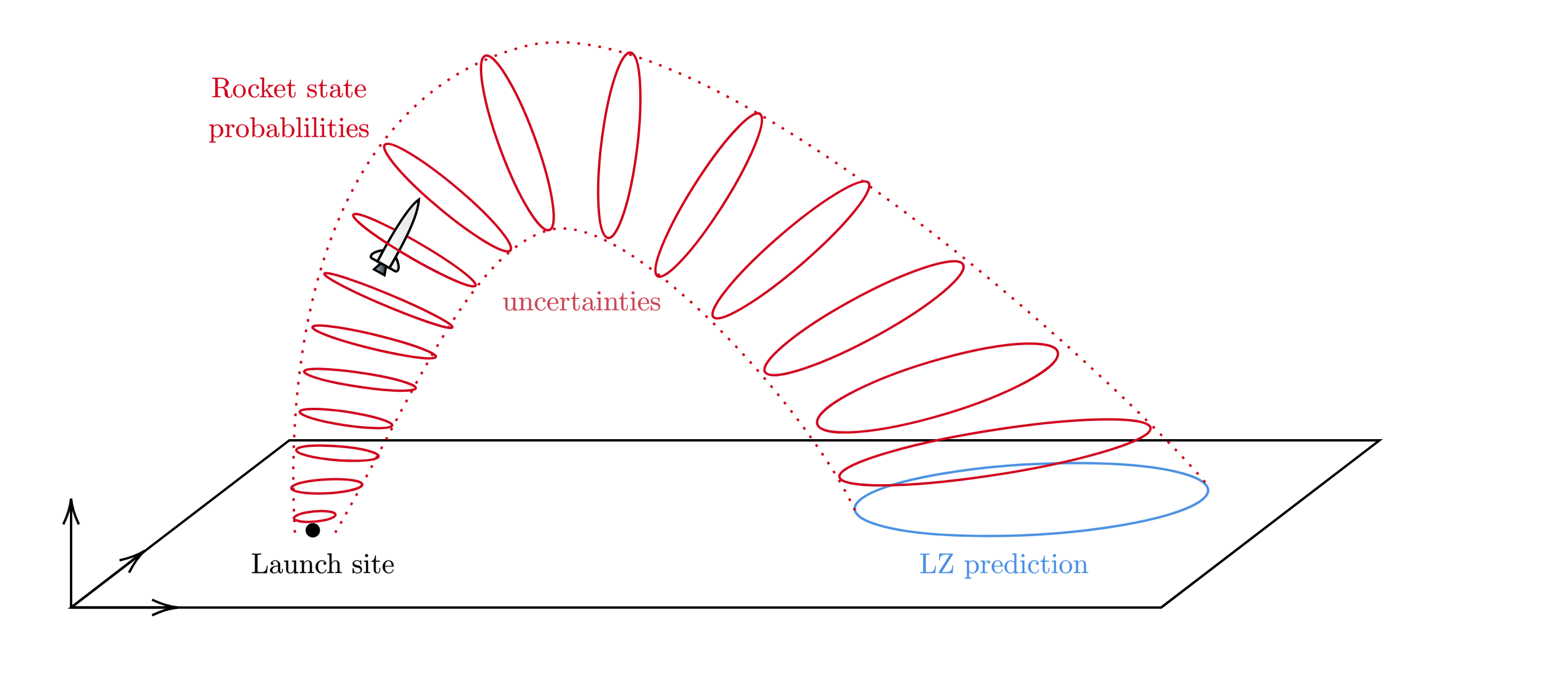
In a rocket trajectory simulation, you're essentially doing a "particle" simulation of a discrete number of particles to know where they may end up after a certain time. You could do this in a continuum by propagating a probability distribution of where the particle could be over time. The dynamics of the distribution is governed by the Fokker-Planck Equation.

PDE Derivation

The dynamics of a rocket with an $n$-dimensional state vector $\mathbf{X}$ is governed by the differential equation: $$\dot{\mathbf{X}}=\mathbf{f}(\mathbf{X}, t) \qquad (1)$$ Where $\mathbf{f}(\mathbf{X}, t)$ is the deterministic system evolution function. Then, by introducing noise (wind gusts, etc.) in the form of a $n$-dimensional Wiener process $\mathbf{W}$, we get a stochastic differential equation of the state vector: $$d\mathbf{X}=\mathbf{f}(\mathbf{X}, t)dt + \mathbf{g}(\mathbf{X}, t)\odot d\mathbf{W} \qquad (2)$$ Where $\mathbf{g}(\mathbf{X}, t)$ is the stochastic system evolution function and $\odot$ denotes the elementwise product. Applying the Fokker-Planck equation to $(2)$: $$\frac{\partial P(\mathbf{X}, t)}{\partial t} =-\frac{\partial}{\partial \mathbf{X}}\left[\mathbf{f}(\mathbf{X}, t)P(\mathbf{X}, t)\right] + \frac{\partial^2}{\partial \mathbf{X}^2}\left[\frac{1}{2}\mathbf{g}^2(\mathbf{X}, t)P(\mathbf{X}, t)\right]$$ We get a partial differential equation in terms of the probability distribution $P(\mathbf{X}, t)$.

Finite Volume Discretisation

We discretise the computational domain into small volumes, and reformulate the dynamics in terms of the probability contained within the volume and how much "flows" out via the boundaries, similar to a finite volume method in fluid dyamics. The insight here is that probability is conserved between volumes. Conservation of probability means that each discrete state-space volume $\Omega$ has a time-change in probability equal to the probability flux $\mathbf{J}(\mathbf{X}, t)$ along the boundary $\partial \Omega$: $$ \frac{\partial}{\partial t} \int_{\Omega} P(\mathbf{X}, t),dV=-\oint_{\partial\Omega} \mathbf{J}(\mathbf{X}, t)\cdot d\mathbf{S}$$ To make our dynamics fit this form, we rewrite The Fokker-Planck PDE in conservative form: $$\frac{\partial P(\mathbf{X}, t)}{\partial t} = \nabla_{\mathbf{x}}^2\left[\tfrac{1}{2}\mathbf{g}^2(\mathbf{X, t})P(\mathbf{X}, t) \right] - \nabla_{\mathbf{x}}\cdot[\mathbf{f}(\mathbf{X}, t)P(\mathbf{X}, t)]$$ We can derive the integral form of the conservative equation using the Divergence Theorem: $$ \int_{\Omega}\frac{\partial P(\mathbf{X}, t)}{\partial t}~dV = \int_{\Omega}\nabla_{\mathbf{x}}^2\left[\tfrac{1}{2}\mathbf{g}^2(\mathbf{X}, t)P(\mathbf{X}, t) \right]~dV - \int_{\Omega}\nabla_{\mathbf{x}}\cdot[\mathbf{f}(\mathbf{X}, t)P(\mathbf{X}, t)]~dV$$ $$\frac{\partial}{\partial t}\int_{\Omega}P(\mathbf{X}, t)~dV = \oint_{\partial\Omega}\left(\tfrac{1}{2}\nabla_{\mathbf{x}}\left[\mathbf{g}^2(\mathbf{X}, t)P(\mathbf{X}, t) \right] - \mathbf{f}(\mathbf{X}, t)P(\mathbf{X}, t)\right)\cdot d\mathbf{S} \qquad (3)$$

Then, we can apply equation $(3)$ to a discrete hypercube in $N$-dimensional state-space (with volume $V$ and wall area $S$). This gives an equation relating the volume-average probability $\overline{P}_{i,j,\dots}$ of a discrete hypercube to the flux across its walls: $$V\frac{\partial \overline{P}_{i,j,\dots}}{\partial t}=S\sum_{n=1}^N\left(\frac{1}{2}\frac{\partial}{\partial x_{n}}\left[g^2_{n}(X_{i,j,\dots}, t)\overline{P}_{i,j,\dots}\right]-f_{n}(X_{i,j,\dots}, t)\overline{P}_{i,j,\dots}\right) $$

Discretizing the spatial derivative as the difference between neighboring volumes:

$$ \overline{P}^{k+1}_{i} = \overline{P}^{k}_{i}\left[1 - \frac{S\Delta t}{V}\sum_{n=1}^N\left(g^2_{n}(X_{i}, t) + f_{n}(X_{i}, t)\right)\right] + \frac{S\Delta t}{V}\sum_{n=1}^Ng^2_{n}(X_{i+1}, t)\overline{P}^k_{i+1}$$

Limitations

From preliminary verification, it became clear that the memory requirements of a simulation would grow exponentially with the dimensionality of the state space, making 3D rigid body simulations computationally intractible. Still, it was a great learning experience.